Deep learning is racking up a serious power bill due to the exponentially increasing number of parameters in modern models. According to an estimate from Strubell et al, training the popular BERT model (more on this below) requires about 1,500 kWh of power over the course of 3 days. That’s about 600 times more electricity than your brain uses in the same time.[1] How can we take a step towards the brain’s efficiency without sacrificing accuracy? One strategy is to invoke sparsity. Today I’m excited to share a step in that direction – a 10x parameter reduction in BERT with no loss of accuracy on the GLUE benchmark.
Sparsity at Numenta
We study sparsity at Numenta because it is a central feature of the brain, with important implications for machine intelligence. If you’re not familiar with sparsity, think of it as meaning “mostly zero”. In the neocortex, neurons form connections to only a small fraction of neighboring neurons, so we say coupling in the brain is sparse. Furthermore, only a small fraction of neurons are active (firing above a given rate threshold) at any given time, so we say activations in the brain are sparse. A sparse neural network is just a neural network where most of the parameters (or weights) are set to 0.
Sparsity confers at least two important benefits: speed and robustness. To increase the speed of neural networks and therefore reduce energy demands, we use a 1-2 punch. First, we “sparsify” and cut down on the number of parameters in the network as much as possible without sacrificing accuracy. Then we implement the sparse network on specialized hardware to deliver a speedup. We’ve demonstrated 20x speedups on CPUs and 100x speedups on FPGAs using neural networks with sparse weights and activations. We’ve also shown theoretically that sparse binary codes are robust to noise, and empirically that this is also true for neural networks with both sparse weights and activations. Recently we even found that sparse activations can help mitigate catastrophic forgetting – another key problem in deep learning today.
BERT and GLUE
Excited by these results, we pursued our goal to build systems that are both fast and accurate by working with a popular type of model in use today: Transformers. We chose BERT[2], a transformer model with 110 million parameters, used on text data. BERT is trained in two phases. In pretraining, you mask words in the text and ask the model to fill in the blank. This is called masked language modeling (MLM). In the finetuning phase, you copy the pretrained model, and add (typically relatively few) training iterations on a new task. The GLUE benchmark consists of 9 finetuning tasks to assess language understanding. The GLUE score averages the success metrics across all 9 tasks.
Pretraining BERT
Sparsifying neural networks is all about balancing sparsity with accuracy. While I mentioned earlier that sparsity has benefits, improper application of sparsity hurts accuracy. The key question is for a given sparsity level, how much accuracy do I need to give up? To answer this question, we pretrained three sparse transformers with 80%, 85%, and 90% sparsity. We relied on a sparsity algorithm that we developed in other projects involving sparse neural networks. After reproducing results from HuggingFace of a GLUE score on the dev set of ~79 after 1 million training steps with a dense model, we decided to save on compute by making all subsequent comparisons at 100k training steps. This lets us get scores that are close to the score after 1 million steps, but at 1/10th the cost. (As a reminder of how expensive the full million steps is, training each model in full takes about as much energy as an Egyptian or Colombian citizen uses in an entire year![3]).
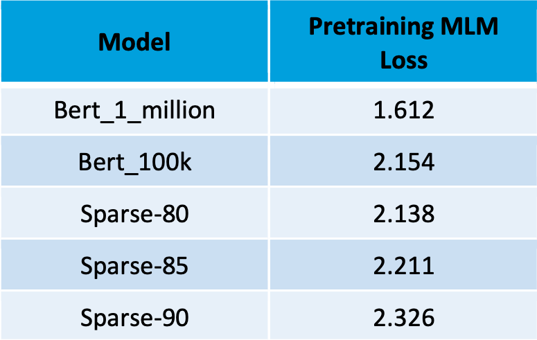
We pretrained each of our four models once on the masked language modeling (MLM) task (see table 1). Differences in the pretraining loss across sparse and dense models at 100k steps were relatively small. If you’re not an ML aficionado, just think of pretraining loss as measuring how bad the model is at the “fill in the blank” pretraining task. The fact that pretraining loss goes down significantly when training for 100k vs 1 million steps is a promising sign for us. It suggests that when we get to the finetuning phase below, we can improve our GLUE scores without any clever business just by training for longer.
Hyperparameter tuning
As a next step, I conducted hyperparameter search for all four models on all nine GLUE tasks. If you’re not familiar with hyperparameter search, I like to think of it as building a customized training protocol for each model. I tuned the learning rate, experimented with learning rate schedulers, and the number of training iterations. We saw a bump in performance on the dev set from anywhere between 1 and 5 GLUE score points for our sparse models.
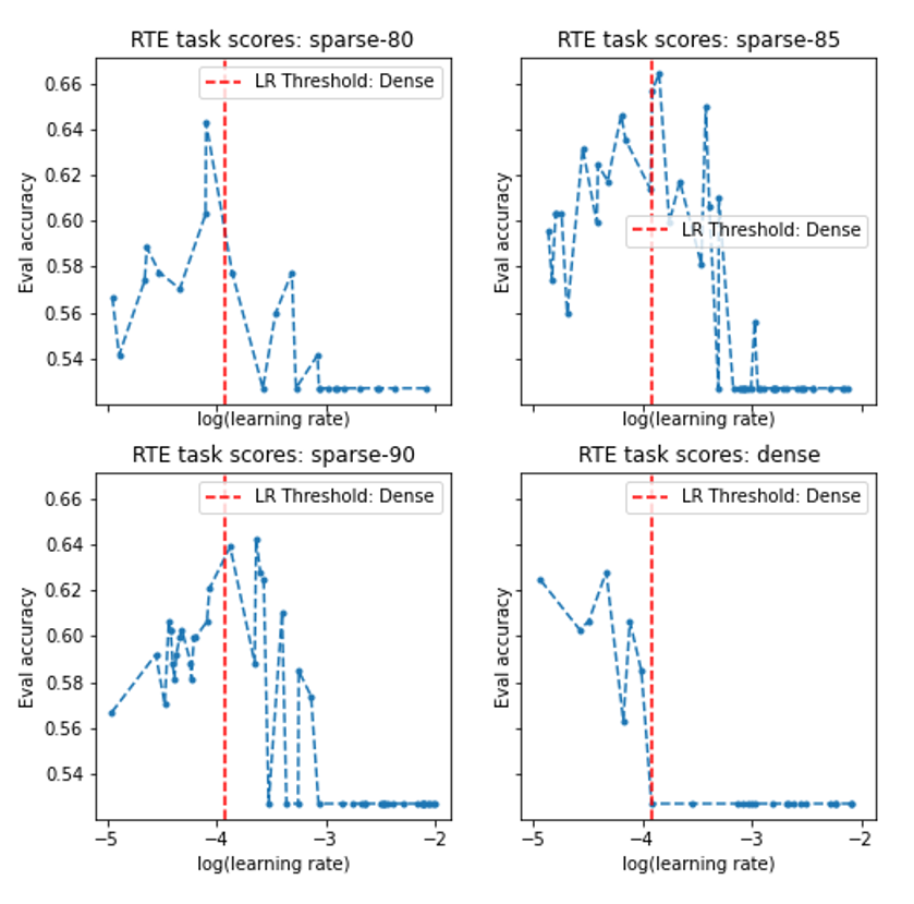
One noteworthy difference we saw between our sparse and dense models was that sparse models tolerated, and indeed benefited from, higher learning rates in the finetuning phase. Figure 1 plots the max accuracy observed during training runs on one of the GLUE tasks in each of the 4 models across the random selection of learning rates used in each case. While the dense model simply crashes when the learning rate exceeds 10e-4, the sparse models perform near-optimally with the same learning rate. The benefits of this robustness to learning rates are twofold. First, the sparse models required fewer trials to find a good learning rate. Second, larger learning rates imply faster finetuning.
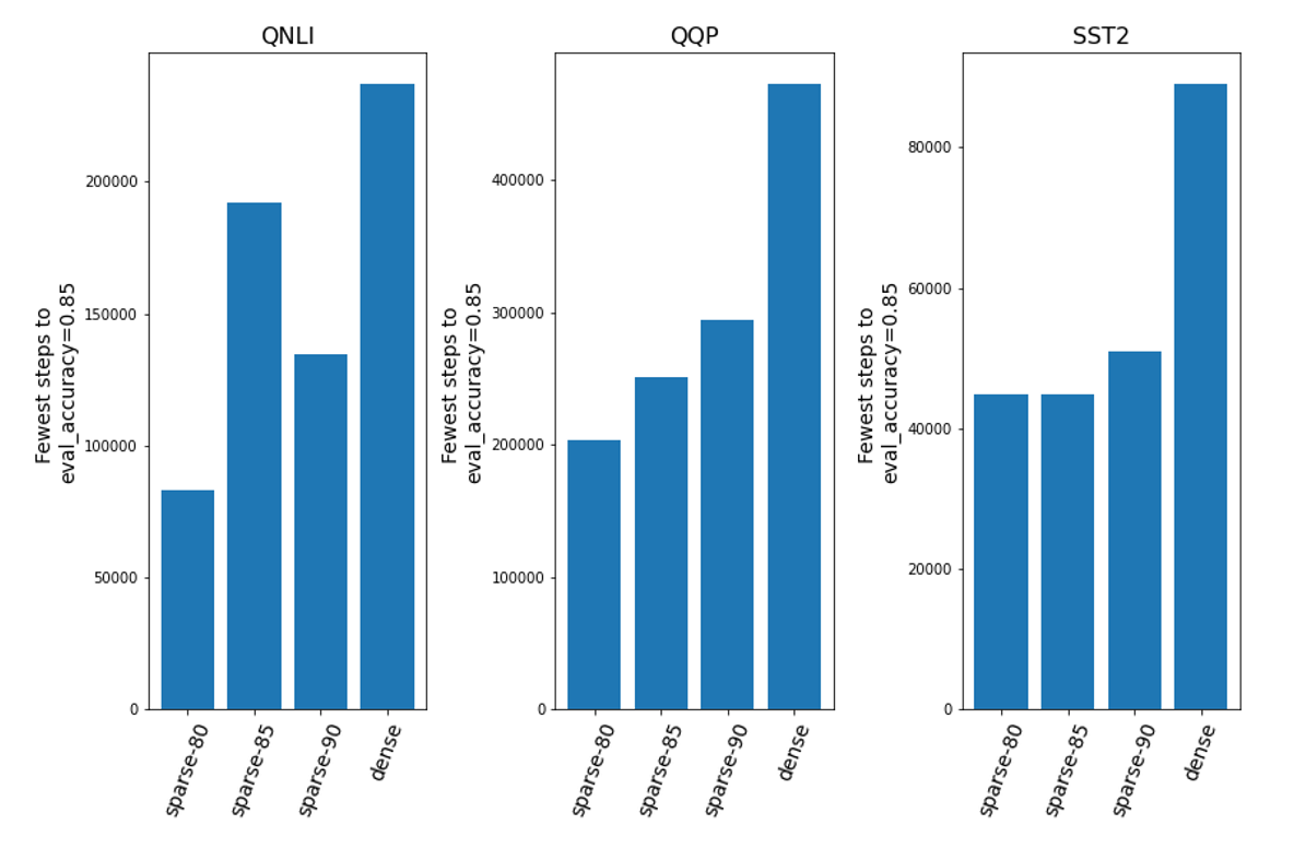
We confirmed this second benefit by calculating how many training steps were needed to reach a given threshold of performance in several GLUE tasks. We selected the fastest time to threshold across all trials for each model. As you can see in Figure 2, the sparse models consistently win the race to threshold. The dense model’s tendency to crash with a higher learning rate explains the initially curious result that hyperparameter search provided a big benefit for sparse models, but very little benefit for the dense. To summarize, the sparse models required less hyperparameter optimization and also converged more quickly during finetuning.
GLUE Scores
To get our final GLUE scores, we conducted multiple training runs for each model and for each task, and selected the best run in each case. The results are in Table 2 below (click on table to expand). The nine rightmost columns are the names of the nine GLUE tasks/datasets, along with the success metrics used for that dataset. Recall that our goal is to compare sparse and dense networks each with 100k pretraining steps. For completeness, we also included our dense model trained for 1 million steps (second row), along with the results from the original BERT paper (first row). Starting with the CoLA column, each column is a natural language understanding task that is named after a dataset. Each of these columns includes one or two measurements of accuracy. Note that in the original BERT paper they did not include scores on the WNLI task, so we term this the BERT score (averaging the metrics for the other 8 tasks).
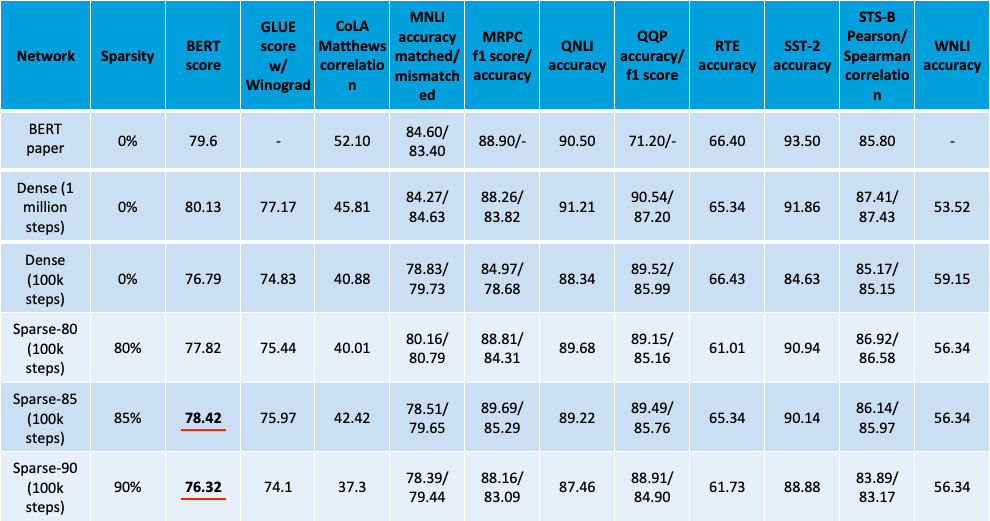
Our sparsest model, with 90% sparsity, had a BERT score of 76.32, 99.5% as good as the dense model trained at 100k steps. Meanwhile, our best model had 85% sparsity and a BERT score of 78.42, 97.9% as good as the dense model trained for the full million steps. These are dev set scores, not test scores, so we can’t compare directly with the results from the BERT paper. Nevertheless, we think these sparse models are competitive with the original paper since the results here have 10% as many training iterations and 10-20% as many parameters (80-90% sparsity).
Conclusion
To summarize the result above, you can remove 9 out of every 10 connections in a transformer and still get GLUE scores that are just as good if not better than the original model. Now that we have a set of transformers that are both sparse and accurate, let’s step back and think about the overall goal again. We are trying to improve the efficiency and reduce the costs of deep learning. Our strategy is to use a 1-2 (sparsity – hardware) punch. The 10x reduction in the number of parameters I presented today is a good start, but it isn’t until the hardware punch lands that we can really drive down energy usage. This is exactly what our architecture team is working on, and we’re hoping to get a proportionate 10x speedup.
If our work sounds interesting and you’d like to collaborate with us, drop us a line at sparse@numenta.com. If you’d like to read more about our recent work, check out the links below. And finally, check out the pretrained models here. We look forward to hearing from you.
- Machine Learning Street Talk Podcast #59 Jeff Hawkins (Thousand Brains Theory)
- Technology Validation: Sparsity Enables 100x Performance Acceleration in Deep Learning Networks
- Fast AND Accurate Sparse Networks
- Can CPUs leverage sparsity?
- Why Neural Networks Forget, and Lessons from the Brain
[1] The brain uses about 20 watts. 20 watts*(1 kilowatt)/(1000 watts)*79 hours ≈ 1.58kWh. If we multiply by the Power Usage Effectiveness coefficient of 1.58 used by Strubell et al, we get ≈ 2.5kWh which is right around 600 times smaller than 1500 kWh. If we don’t take this multiplicative constant into account, the ratio goes up to 1500kWh/1.58kWh ≈ 950.
[2] Note that throughout this blog, BERT refers to BERT-base, not BERT-large.
[3] Using Strubell’s estimate of 1500kWh, and Wikipedia’s listing of kWh per capita of various countries. The cost is in the thousands if you prefer units of USD!