
About a year ago, in the post The Case for Sparsity in Neural Networks, Part 1: Pruning, we discussed the advent of sparse neural networks, and the paradigm shift that signals models can also learn by exploring the space of possible topologies in a sparse neural network. We showed that combining gradient descent training with an optimal sparse topology can lead to state of the art results with smaller networks. In the brain, sparsity is key to how information is stored and processed, and at Numenta we believe it to be one of the missing ingredients in modern deep learning.
We define a sparse neural network as a network in which only a percentage of the possible connections exists. You can imagine a fully connected layer with some of the connections missing. The same can be extended to several other architectures, including ones in which the weights are reused, such as CNNs, RNNs or even Transformers.
Previously, we discussed pruning post training as one way of getting sparse neural networks. But although pruning delivers the speed and size benefits of sparse networks for inference, the training cost is usually higher. It requires training a dense network prior to pruning plus additional cycles of fine tuning in order to reach the same level of accuracy of regular dense networks.
What if we could train sparse networks from scratch without compromising accuracy? That is what we will cover in this post, reviewing some of the latest contributions in the literature.
Dynamic sparse algorithms
While pruning converts a trained dense network into a sparse one, there are several methods of training neural networks which are sparse from scratch, and are able to achieve comparable accuracy to dense networks or networks pruned post training. This general class of algorithms has come to be known as dynamic sparse neural networks.
One of the earliest papers proposed Sparse Evolutionary Training (SET), a very simple yet surprisingly effective algorithm. In SET, a neural network is initialized at a given sparsity level, with the set of sparse connections decided randomly. At the end of each epoch, 30% of the existing connections with the lowest absolute magnitude (15% of the lowest positive and 15% of the lowest negative) are pruned, and new random connections are allowed to grow in its place.
SET works well for some supervised learning problems, and it laid the groundwork for dynamic sparse algorithms that would follow. In practice, however, SET doesn’t scale well to larger models and datasets. One of the issues seen here and in some of the later algorithms is how to protect the newborn connections from being pruned again in the next round, given newly grown connections are initialized with zero weight. Another important issue is efficiency, considering ranking is done by magnitude and requires sorting all the weights at each epoch.
Aiming to solve some of these issues, Mostafa and Wang were able to extend SET to a bigger class of problems, such as ImageNet, with a few simple modifications. In their algorithm, Dynamic Sparse Reparameterization, weights are pruned based on a threshold, and the threshold is increased or decreased depending on whether the number of weights pruned at the last step was higher or lower than expected. The threshold is global, one for the entire network, allowing the sparsity level to fluctuate between layers.
The free reallocation of parameters between layers has proven to be paramount to an effective dynamic sparse algorithm. Several methods that followed kept that approach, but experimented with other ways of deciding which connections to prune or which connections to add. As our own exploration shows, the layers of a neural network have different relevance, measured by accuracy on the test set.
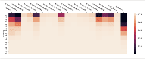
The heatmap shows the impact on the model accuracy of pruning a Resnet50 trained on Imagenet, each block at a time (the rightmost column is pruning the full model). As sparsity increases, the impact to accuracy increases correspondingly. The pattern is similar to the one seen in Are All Layers Created Equal?, where the authors reinitialize the weight to a certain epoch instead of pruning. The biggest impact comes from pruning the earliest and the latest blocks, including the first block of each Resnet stage.
In Sparse Networks From Scratch: Faster Training without Losing Performance, the weights are redistributed according to the mean momentum magnitude of each layer. This paper introduces the use of momentum (a moving average of gradients) as an additional saliency metric to decide which connections to prune or grow. Their experimental results show that while momentum is useful in pruning, it does not help in deciding which connections to add back into the network, failing to outperform random selection.
A more recent paper was able to use the gradient information effectively to guide growing connections. Rigging the Lottery Ticket, from Google Brain’s research team, gained a lot of attention and showed state of art results in dynamic sparsity. The algorithm keeps track of the gradients even for dead neurons and the connections with the highest magnitude gradient are grown back into the network. This method holds some similarities to Sparse Networks from Scratch, but it achieves increased efficiency by calculating the gradients in an online manner and storing only the top-k gradient, while also showing improved results.
Many similar papers in the domain of dynamic sparsity were published in the past year, with a last special mention to Winning the Lottery with Continuous Sparsification. And we are certain that many more will come once the benefits of training sparse networks are fully realized by the community and supported by the existing hardware solutions.
Foresight pruning
In addition to sparsity during training, can we go even further, and find the optimal set of connections even before we start training? A class of algorithms known as foresight pruning have attempted to achieve just that. Published in 2018, Single Shot Network Pruning (SNIP) introduced a new saliency criteria that measures how relevant a connection is to training the network, based on its influence on the loss function. This is calculated through a sensitivity analysis that measures the rate of the change of the loss function with respect to a change in each connection. This new saliency criteria, named connection sensitivity, achieves up to 99% sparsity with only marginal increase in the error in simple networks and datasets.
One of the critiques of SNIP is that it is dependent on the dataset, and doesn’t create generalizable sparse architectures. A more recent paper from Surya Ganguli’s group looks at the problem from a different angle. The authors seek to avoid two known issues from earliest foresight pruning algorithms: removing dependency from data, and avoiding layer collapse. Their algorithm, Synaptic Flow Pruning, aims to preserve the flow of synaptic strengths through the network at initialization. Improving the gradient flow is also employed by Gradient Signal Preservation (Grasp), which achieves up to 80% sparsity in Imagenet trained networks with very little loss in accuracy.
There are two ways these techniques can be combined with dynamic sparsity. Instead of deciding the initial connectivity randomly, we can apply a foresight pruning algorithm to set the initial topology and then evolve it through dynamic sparse algorithms. But once the network starts learning, the initial conditions that were optimized for better gradient flow are no longer guaranteed. One way around this is to incorporate gradient flow as another saliency metric in dynamic sparsity. Lee et al. who further explore this signal propagation perspective to pruning, propose in future work that such algorithms can be used to rebalance the connections and maintain signal propagation at an optimal level throughout training.
Last month a paper released by the authors of the Lottery Ticket shows that in all the foresight pruning methods cited above, if the sparse connections are randomly permuted within each layer, the trained model achieves the same level of accuracy or above. The implication is that the only true advantage in these methods is in deciding the degree of sparsity per layer, going back to the same conclusion we first had when analyzing dynamic sparse algorithms. If the results hold, it is an invitation to rethink foresight pruning algorithms. It is an early area of research, but with a lot of potential to grow.
The implications to hardware
One immediate benefit of sparse neural networks is smaller size, given we only need to keep the non-zero connections, which is a huge benefit when trying to fit the networks in edge devices. The sparse network is compressed in the same ratio as the amount of sparsity introduced. But other than the size, in traditional hardware it is hard to extract any additional benefits of sparse networks. In GPUs it is usual to fill in missing connections with zeros to perform matrix products, so the benefits of sparse matrices are not translated into added efficiency in the forward or backward pass.
Manufacturers have been keenly aware of that. The market leader in GPUs, NVIDIA, recently published a thorough study of sparse neural networks, noticing the increase in importance in this research area in the past years. The newly released chip Ampere has some limited support for sparsity that may help close that efficiency gap.
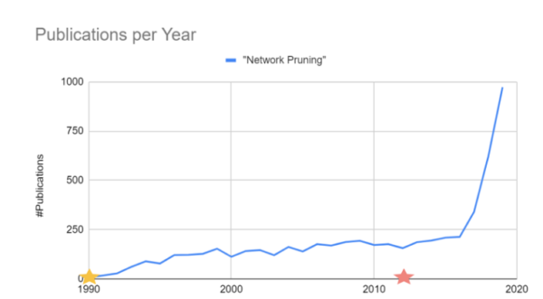
Number of publications citing network pruning per year. Source: Accelerating Sparsity in NVIDIA Ampere (2020)
Other hardware startups have emerged with a full focus on sparsity, such as Graphcore IPUs, that promise a 5x speedup compared to traditional GPUs. Cerebra called their main computational unit a Sparse Linear Algebra Compute (SLAC), and have been actively working in adapting hardware to handle sparse neural networks. FPGA chip makers are also well positioned to deal with this new requirement due to the flexibility of their hardware and a longtime focus on compression and efficiency on the edge.
As Sara Hooker points out in The Hardware Lottery, the research direction is inevitably influenced and limited by the tools we have available to run our algorithms. In the past decade we’ve seen back propagating dense networks thrive in the era of GPUs. If a new wave of sparse optimized hardware emerges, will we be looking at sparse neural networks as the new paradigm for large scale deep learning?
Sparse activations and beyond supervised learning
Up until now we have only talked about sparsity in weights. But another relevant theme is neural networks with sparse activations. The benefits of combining sparse activation with sparse weights are huge. If the output of a layer is 20% sparse, and the weights to the next layer are also 20% sparse, the number of non-zero multiplications is only around 4%. If we can take advantage of non-zero multiplications at a hardware level, this represents a 25x times gain in speed compared to regular networks.
In our last post of this series, we will dive into more details of some of the research we’ve been doing at Numenta regarding sparsity activations and some of the most recent findings in the literature. We will also look into applications of sparse neural networks in other fields beyond computer vision and supervised learning. See you soon!