
Last week at Numenta we held our monthly Brains@Bay meetup, gathering data scientists and researchers in the Bay Area to talk about Sparsity in the brain and in Neural Networks (recordings available here). Sparsity is a topic we’ve also been extensively discussing in our research meetings and journal clubs in the past weeks.
Sparsity has long been a foundational principal of our neuroscience research, as it is one of the key observations about the neocortex: everywhere you look in the brain, the activity of neurons is always sparse. Now as we work on applying our neuroscience theories to machine learning systems, sparsity remains a key focus. There are so many different aspects to it, so let’s start at the beginning. In this blog post, I’ll share my summary of literature review on the topic of pruning.
The dawn of pruning
The story of sparsity in neural networks starts with pruning, which is a way to reduce the size of the neural network through compression. The first major paper advocating sparsity in neural networks dates back from 1990, written by LeCun and colleagues while working at AT&T Bell Laboratories. At the time, post-pruning neural networks to compress trained models was already a popular approach. Pruning was mainly done by using magnitude as an approximation for saliency to determine less useful connections – the intuition being that smaller magnitude weights have a smaller effect in the output, and hence are less likely to have an impact in the model outcome if pruned. In Optimal Brain Damage, LeCun suggested different metrics could be a better approximation to saliency, and proposed using the second derivative of the objective function with respect to the parameters as a pruning metric.
This paper jumpstarted the field of neural network pruning, with important developments being made in the following years. Compressed models became even more important with the rise of the Internet of Things. As machine learning models were pushed into embedded devices, such as smart cameras able to recognize visitors at your front door and irrigation devices that can automatically adjust the flow of water and maintain optimal conditions for crops, compressing neural networks grew in importance.
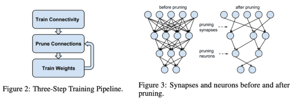
In 2015 Han et al. published a now highly cited paper proposing a three step method to prune neural networks: 1) train a dense network; 2) prune the less important connections, using magnitude as a proxy for saliency; 3) retrain the network to fine-tune the weights of the remaining connections. Surprisingly, they showed this method was not only comparable to regular deep learning models, but could achieve even higher accuracy.
Finding the lottery ticket
This post-pruning technique has been widely used and improved upon, and considered to be the state of the art until very recently. But the burgeoning question was, why does it work so well?
Some researchers set out to investigate the problem and answer the question. Most notably, Frankle and Carbin (2019) found out that fine-tuning the weights after training was not required for these new pruned networks. In fact, they showed the best approach was to reset the weights to their original value, and then retrain the entire network – this would lead to models with even higher accuracy, compared to both the original dense model and the post-pruning plus fine-tuning approach proposed by Han and colleagues.
This discovery led them to propose an idea considered wild at first, but now commonly accepted – that overparameterized dense networks containing several sparse sub-networks, with varying performances, and one of these sub-networks is the “winning ticket” which outperforms all others. The DL research community quickly realized they were onto something, and several approaches for finding this winning ticket have been proposed to date.
Different points of view
But the story doesn’t end there. A concurrent paper by Liu et al., tried to replicate the results, but using structured pruning approaches instead of unstructured pruning. Structured pruning means pruning a larger part of the network, such as a channel, or a layer. Unstructured pruning, on the other hand, is what we have been discussing so far – find the less salient connections, and remove them, wherever they are. The disadvantage with the latter is that the sparse networks created by unstructured pruning don’t have obvious efficiency gains when trained in GPUs.
Going back to Liu et al., they found that for all major structured pruning approaches it would be better to retrain the pruned network instead of fine-tuning the end state of the trained dense network. However, they came to a different conclusion than Frankle and Carbin: the pruned model would have equivalent performance of a dense model, even if the weights are randomly reinitialized. Resetting the weights to their initial values was as good as reinitializing them to random values.
That would lead them to conclude that structured post-pruning is doing something similar to neural architecture search, finding the optimal architecture that works better for the given problem. The difference lies in that, in architecture search paradigms, you start with the minimal network possible and build from the ground up. In structured pruning, on the other hand, you start with a large dense network and prune it after training to achieve the smallest possible network which has similar or superior performance compared to the dense network.
The story, however gets even more interesting. Research published in an ICML workshop shortly after, by Zhou et al. from Uber AI, runs several experiments on the lottery ticket (LT) algorithm and discovers something even more remarkable. First, they break down the value of a weight into two components, its sign (+ or -) and magnitude. Then, they reinitialize the pruned network weights to the same sign of their original weights, but with their magnitude set to a fixed constant (all weights are set to the same magnitude). Surprisingly, this method allows pruned models to outperform their dense counterparts, with results comparable to the LT algorithm. A second experiment in the same paper shows something even more remarkable: without any re-training, this reinitialized pruned model can achieve up to 84% accuracy on MNIST!
How relevant are learned weights?
Before we conclude, let’s look at further evidence. Gaier and Ha, at Google Brain, conceived an interesting experiment. Using evolutionary algorithms, similar to the ones used in traditional neural architecture search, they evolved architectures from the scratch to optimize for both number of parameters and performance on the task. Their goal was to create the smallest network capable of solving the problem as well as regular state-of-the-art networks. But, in an interesting twist, they decoupled the problems of learning the architecture and learning the weights by using one predefined weight as the single parameter shared by all the connections. With this trick, the researchers were able to evaluate the architecture independent of the weights. The networks grown by this model did not achieve state of the art results – however, they performed approximately 10x better than randomly initialized networks at RL tasks, and 15x better if the single shared weight was optimized as well (in comparison, fully dense networks perform 20x better than random in the same task).
Also at Google, Zhang et al. (2019) analyzed several trained convolutional neural networks to understand if every layer has a similar influence in the network’s output. For each layer, one at a time, they reinitialized all the weights either to their initial value (prior to training) or to a random value, and evaluated how much that change impacted the output. The experiments showed that, for deep networks, reinitializing the weights of hidden layers in the middle of the network would have no impact at all on the results – only the weights in the initial or final layers of the network really matters. To explain that phenomenon, Zhang et al. raise the hypothesis that overparameterized deep networks automatically adjust their de-facto capacity by relying on some connections (or in this case some layers) more than others.
Are there other benefits for sparsity?
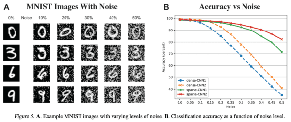
Yes! The inspiration for sparse networks in machine learning comes from the brain, and several other properties related to how humans learn can be associated with sparsity. One of them is robustness. As we showed in 2016 (Ahmad & Hawkins, 2016), sparse representations are naturally more robust to noise. These findings are easily extendable to deep learning architectures, as described in our most recent work. A sparse set of connections coupled with a sparse activation function, such as winner-take-all, lead to very sparse neural networks which outperforms dense networks in test sets modified by adding white noise.
Sparse models might also be a better fit to continuous or lifelong learning, i.e. learning continuously using the same network even when tasks and the underlying statistics change (see Cui et al., 2016). We’ve discussed above the hypothesis of a dense network being composed of several sparse sub-networks. Each of these sparse sub-networks could be trained to learn a specific task, as recently proposed in a paper by Golkar et al. (2019).
Research directions
The pruning literature have shown sparse models outperform dense models, but in order to find the optimal set connections that compose the winning ticket model, they suggest we need first to train a dense model. This leads to efficiency gains in inference, but not in training.
What if we can find the winning ticket without training a dense model? Is there a way of a training a sparse network to learn the optimal set of connections during the regular training pass, so we can have sparse models during training as well? We leave that to the next post.